Your Starting Salary Matters More Than You Think: A Deep Dive into Income Analysis
Introduction
When you’re applying for a job one of the most important topics is probably going to be how much you’re going to get paid for your work. An employer offers you a number after which you either accept, reject or, if you’re really daring, you bargain which may result in you getting higher pay or some additional benefits.
Lately, my friends and I had big disputes over this topic. I was seeking a new job and had rejected multiple employers because of the unacceptably low compensation which doesn’t even cover basic life expenses. The arguments my friends gave me were along the lines of:
“You’ve got to start from somewhere.”
“The economy is not the best so be happy that you even got the offer.”
“It’s IT, salaries grow fast.”
“Better something than nothing.”
To my surprise, many had shared the same thinking even though I didn’t have insanely high expectations but rather a slightly above average salary (for our country, that is).
Even though their arguments were somewhat valid, and us talking about it wasn’t going to change anything, I just couldn’t make peace with the whole situation. That’s what motivated me to do a bit of analysis with some highschool maths.
Mathematical Models
Let’s consider a few possible scenarios:
- Ana (A) has a constant salary (\(B_{const}\)) and never gets a raise.
- Bob (B) gets a salary percentage increase. Meaning every \(l_{raiseFreq}\) months, the salary from the previous month gets multiplied by a percentage \(p\), with a base/starting salary of \(B_{0}\).
- Chris (C) gets a constant salary increment periodically. Meaning every \(l_{raiseFreq}\) months, the salary from the previous month increases by an amount of \(c_{inc}\), with a base/starting salary of \(B_{0}\).
where \(x\) is a variable of time in months and \(B_{const},\ B_{0},\ l_{raiseFreq},\ c_{inc},\ p\) will be fixed parameters for each of the graphs.
These formulas can probably be rewritten to be more concise but I left them in this form because I feel this is how most people would do it on paper.
What are these formulas actually?
It may not be clear why I chose these models (A, B, C), but all of them were chosen to reflect real life situations.
Linear model (A)
The simplest model is representing a boss that never gives Ana more than she already has. While mostly uncommon in real life situations, this will serve as a great “control group”.
Example for a 6 month period with a salary of 1500:
\[ \begin{aligned} A(6) &= 1500 \cdot 6 \\ &= 1500\ +\ 1500\ +\ 1500\ +\ 1500\ +\ 1500\ +\ 1500\\ &= 9000 \end{aligned} \]yields an income of 9000.
Geometric progression (B)
This is probably the most common form of getting a raise. The employer offers Bob a 12% increase on his current salary, or in other words his new salary will be the current salary multiplied by 1,12.
Example for a 18 month period with a starting salary of 1000 and a percentage increase of 12% every 6 months:
\[ \begin{aligned} B(18) &= 6 \cdot 1000 \cdot 1.2^0\ +\ 6 \cdot 1000 \cdot 1.2^1\ +\ 6 \cdot 1000 \cdot 1.2^2\\ &= 6 \cdot 1000\ +\ 6 \cdot 1200\ +\ 6 \cdot 1440\\ &= 21,840 \end{aligned} \]yields an income of 21,840, and the final salary of 1440.
Arithmetic progression (C)
The chief gives Chris a constant amount increase every time they have the periodic review. This means that the first raise may be a significant boost to his salary, but after a couple of such raises it will have less of an effect. For example, adding 300 to 1000 is a generous increase of 30%, but adding 300 to 3000 is only 10%!
Example for a 18 month period with a starting salary of 1000 and a constant amount increase of 300 every 6 months:
\[ \begin{aligned} C(18) &= 6 \cdot (1000\ +\ 0 \cdot 300)\ +\ 6 \cdot (1000\ +\ 1 \cdot 300)\ +\ 6 \cdot (1000\ +\ 2 \cdot 300)\\ &= 6 \cdot 1000\ +\ 6 \cdot 1300\ +\ 6 \cdot 1600\\ &= 23,400 \end{aligned} \]yields an income of 23,400, and the final salary of 1600.
Salary analysis (graph)
My analysis was done using an online math tool Desmos so feel free to follow along if the images are not clear. When you get a grasp of what’s going on, you can even change the parameters to do the analysis yourself. For now, it’s important to note that the x axis is representing the number of months while the y axis is representing the amount of income accumulated over \(x\) months. Blue graph represents Ana’s income, red is Bob and green is Chris.
The models can be analyzed in two ways:
- Compare each of them graphically to get a visual picture on how fast they accumulate income compared to each other
- Calculate how much income each of them yields after a period of time
Both Bob and Chris will get their salary increase in periodic intervals which accurately reflects real life.
Considerations
Comparing the models (with the same base salary), it’s obvious that model A will perform the worst, whereas the performance of models B and C will depend on the aforementioned parameters. We could analyse which of the two is better but I think it can portray a wrong picture about the real life situation. Taking into account that our time interval is limited (not planning to work forever), salaries usually hit a ceil at some point (don’t expect to get a raise beyond a certain point) and performance of both models strongly depends on the parameters (Bob having a 5% periodical increase will have a very slow progression compared to Chris getting 300 increase flat).
To better portray differences between each of the graphs, some of the parameters will stay fixed and x and y coordinates will stay in the same range. There’s no point in letting Ana have the same starting salary as Bob and Chris so let’s level the playing field. Ana gets a salary of \(B_{const}=1500\), Bob and Chris start from \(B_{0}=1000\) and they get a raise every \( l_{raiseFreq}=6\) months.
Optimistic case (high increase)
First, let’s assume Bob and Chris have a great boss. Bob is boosted by 20% (\(p=1.2\)) while Chris gets a bump of \(c_{inc}=300\). Remember, that’s an increase after every six months as stated in the previous paragraph.
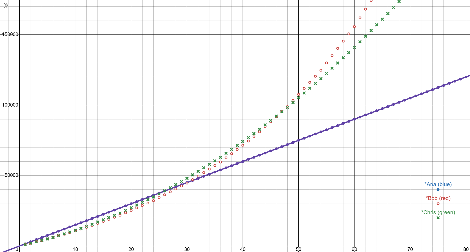
It’s easy to notice that both Bob and Chris surpass Ana, but the interesting part is the amount of time required for that to happen. After 25 months, Chris will have gotten a raise four times, ending up with a salary of 2200, but still with less money on his account than “poor” Ana. Bob will end up on top, but only after 4 years of getting raises semiannually.
Realistic case (medium increase)
In this case, Bob and Chris get an increase of (\(p=1.12\)) and \(c_{inc}=200\) respectively. This is a more realistic situation of a good salary increase in the real world. One that many people are usually satisfied with.
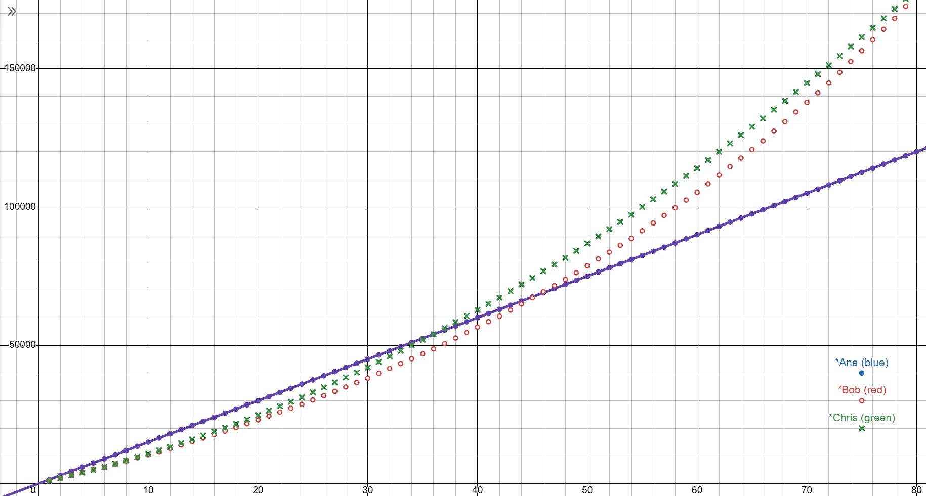
Bob will have more money than Ana after 46 months and Chris will take exactly 3 years. By some statistics, this is how long most people stay in a company before finding another one.
Usual case (low increase)
Lastly, this case portrays the reality most people have to deal with. An increase of 6% (\(p=1.06\)) or an additional \(c_{inc}=100\) on their salary.
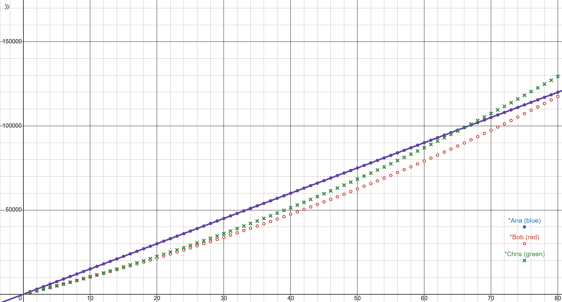
By the time Bob and Chris catch up to Ana, most people start switching careers. It takes Bob 7 years to accumulate more than Ana and Chris is going to get there in 5 and a half years .
Comparative analysis
Let’s recap! Ana didn’t get any salary increase but spends most of the time with more money then Bob and Chris. This showcases how important it is to negotiate the first salary well, like Ana did, because you will probably end up getting at least some salary increase over the years which extends the intersection of these graphs even more. You might have a bigger salary than your colleagues but it will take you years to catch up to the amount of income they accumulated if you started with a significantly lower salary.
Another interesting but hidden fact is that comparisons between graphs are preserved regardless of the base salaries, given that the salaries have the same ratio. What I mean by this is that Bob will require the same number of months to catch up to Ana if the salaries are \(B_{const}=1500, B_0=1000\) or if they are \(B_{const}=2100, B_0=1400\). The ratio in this case is 50% difference (\(B_{const}=1.5 \cdot B_0\)) since Geometric progression increases exponentially. Likewise, Chris will take the same amount of time to catch up to Ana no matter if the salaries are \(B_{const}=1500, B_0=1000\) or if they are \(B_{const}=2100, B_0=1600\). In this case the ratio is the exact amount difference (\(B_{const}=B_0\ +\ 500\)) since Arithmetic progression increases linearly.
Income yield analysis
These graphs are also excellent to put yourself in the position of the employer in case you were thinking about starting your own business, though it’s necessary to do some additional calculations when accounting for taxes.
Since it’s post Christmas time, you may want a nice way to visualise a common business trick: how big of a bonus you would need to get to catch up to Ana. To do that, we just compare the “gap” between the graphs. Check how much we would need to add to Bob’s income for the graph to intersect with Ana’s income. What may be surprising is that getting bonuses multiple times a year will (usually) still yield less income than just having a higher salary.
Taking optimistic case as an example, Bob would have a salary of 1728 but he would still need more than two and a half salaries of bonus to catch up to Ana’s income.
Also it’s worth noting, while the salary is guaranteed, the bonuses are not.
Conclusion
If you’re a young person such as myself, it’s much more important to have a better start and lower salary growth than the other way around. There are multiple reasons for that but one of the more obvious ones is that we don’t own anything yet which means that we have a lot of things to buy out of necessity which may require mortgages which lower the total income, prolonging the time it takes to achieve Ana’s income level.
By settling on a lower pay you are relying on the fact that your employer will give frequent raises, whereas starting with a higher salary provides you with a clear picture of your financial situation.
After attending many interviews recently, I’m glad I didn’t settle for less, as accepting those offers would have contributed to normalizing the underpayment of those who may not have the option to refuse. By rejecting offers that didn’t even cover basic living expenses, I hope to encourage employers to reconsider and offer fairer compensation to other candidates.